摩拜單車資料探索
探索背景
摩拜單車舉行過一個演算法挑戰賽,給出了一個包含300多萬條在北京產生的訂單資料csv檔案(資料鏈接)
其資料形式如下:

資料後兩列分別是起始點與結束點的7位geohash值,即經過geohash編碼過的經緯度。其值位數越多越精確,每個值相同部分越多越鄰近,7位程式碼誤差大概為76m。
分析猜想
資料來自於共享單車,把共享單車這一功能性作為切入點,不妨大膽作以下猜想:
1。共享單車為解決人們“最後一公里”的需求應運而生,所以總體平均路程應該是在1公里左右;
2。如果用使用6位geohash切分,一個區域大概是0。34平方千米,誤差大概是610m,基於第1點,大部分訂單應該是從一個區域出發到鄰近的區域去;

6位geohash示意圖
3。從時間上看,訂單產生應該集中在工作日早晚上下班的時間段,在居住地和地鐵,公交站間來回。
資料處理
基於以上以上三點猜測,需要對資料進行相應處理:
#匯入關鍵的包
from math import radians, cos, sin, asin, sqrt
import pandas as pd
import seaborn as sns
import geohash
import matplotlib。pyplot as plt
%matplotlib inline
train = pd。read_csv(“train。csv”,sep = ‘,’,parse_dates=[‘starttime’])
#資料處理函式
def _processData(df):
# Time處理
#0~6分別代表星期日~星期六
df[‘weekday’] = df[‘starttime’]。apply(lambda s : s。weekday())
df[‘hour’] = df[‘starttime’]。apply(lambda s : s。hour)
df[‘day’] = df[‘starttime’]。apply(lambda s : str(s)[:10])
print(“Time process successfully!!!”)
# 7位Geohash解碼——>(維度,經度)
df[‘start_lat_lng’] = df[‘geohashed_start_loc’]。apply(lambda s : geohash。decode(s))
df[‘end_lat_lng’] = df[‘geohashed_end_loc’]。apply(lambda s : geohash。decode(s))
#擷取6位geohash
df[‘geohashed_start_loc_6’] = df[‘geohashed_start_loc’]。apply(lambda s : s[:6])
df[‘geohashed_end_loc_6’] = df[‘geohashed_end_loc’]。apply(lambda s : s[:6])
df[‘start_neighbors_6’] = df[‘geohashed_start_loc_6’]。apply(lambda s : geohash。neighbors(s))
print(“Geohash process successfully!!!”)
# 判斷目的地是否在neighbors
def inGeohash(start_geohash,end_geohash,names):
names。append(start_geohash)
if end_geohash in names:
return 1
else:
return 0
df[‘inside_6’] = df。apply(lambda s :inGeohash(s[‘geohashed_start_loc_6’],s[‘geohashed_end_loc_6’],s[‘start_neighbors_6’]),axis = 1)
print(“Geohash inside process successfully!!!”)
# 起始點到結束點的直線
def haversine(lon1, lat1, lon2, lat2):
“”“
Calculate the great circle distance between two points
on the earth (specified in decimal degrees)
”“”
lon1, lat1, lon2, lat2 = map(radians, [lon1, lat1, lon2, lat2])
# haversine公式
dlon = lon2 - lon1
dlat = lat2 - lat1
a = sin(dlat/2)**2 + cos(lat1) * cos(lat2) * sin(dlon/2)**2
c = 2 * asin(sqrt(a))
r = 6371 # 地球平均半徑,單位為公里
return c * r * 1000
df[“start_end_distance”] = df。apply(lambda s : haversine(s[‘start_lat_lng’][1],s[‘start_lat_lng’][0],s[‘end_lat_lng’][1],s[‘end_lat_lng’][0]),axis = 1)
print(“Distance process successfully!!!”)
return df
train = _processData(train)
一通操作下來,得到新的train應該是在原有的基礎上多瞭如下的項:

資料分析
先來看看騎行距離的五數概括:

可以看到平均里程是814米,與我們預想的比較接近。
至於這個最大值。。。

將近45公里,可能是被一個吃了炫邁的騎行愛好者翻牌了,也可能是裝置出現故障。
統計下有多少訂單在開始區域的九宮格範圍內

大概81。45%騎行到鄰區
然後看總體訂單量按時的分佈情況:

可以看出訂單量最密集的時間是在早7,8點和晚5,6點,基本符合我們的猜想。
再看看工作日與非工作日之間有哪些差別:
在此之前,需按照day列劃分工作日與非工作日,分別統計兩者每小時的訂單量平均值,為此需定義一個函式:
def
_timeAnalysis
(
df
):
# 週一 至 週日 不同時間的用車
df
。
loc
[(
df
[
‘weekday’
]
==
5
)
|
(
df
[
‘weekday’
]
==
6
),
“isWeekend”
]
=
1
df
。
loc
[
~
((
df
[
‘weekday’
]
==
5
)
|
(
df
[
‘weekday’
]
==
6
)),
“isWeekend”
]
=
0
g1
=
df
。
groupby
([
“isWeekend”
,
‘hour’
])
# 計算工作日與週末的天數
g2
=
df
。
groupby
([
“day”
,
“weekday”
])
w
=
0
# 週末天數
c
=
0
# 工作日天數
for
i
,
j
in
list
(
g2
。
groups
。
keys
()):
if
j
>=
5
:
w
+=
1
else
:
c
+=
1
#
temp_df
=
pd
。
DataFrame
(
g1
[
‘orderid’
]
。
count
())
。
reset_index
()
temp_df
。
loc
[
temp_df
[
‘isWeekend’
]
==
0。0
,
‘orderid’
]
=
temp_df
[
‘orderid’
]
/
c
temp_df
。
loc
[
temp_df
[
‘isWeekend’
]
==
1。0
,
‘orderid’
]
=
temp_df
[
‘orderid’
]
/
w
(
temp_df
。
sort_values
([
“isWeekend”
,
“orderid”
],
ascending
=
False
))
sns
。
barplot
(
x
=
‘hour’
,
y
=
“orderid”
,
hue
=
“isWeekend”
,
data
=
temp_df
)
結果如下圖:

可以看到,在訂單量的比較中,週末的分佈比較均勻,當初工作日起的早早的人也小睡了一下懶覺。
出發點和目的地:
先把7位geohash轉換成經緯度,得到起始和結束的經緯度,然後按訂單量選取前二十,如下圖:
得到流向圖如下:


flowmap預覽
詳細連結為:前20
透過放大觀察可知這些軌跡有一個共同點,就是一個在住宅區,一個在地鐵站附近,說明摩拜單車很好地履行了它幫助人們完成最後一公里的使命。
下一篇:更換桑塔納空調濾芯